Logical/physical operators

Logical operators
                what they do
                e.g., union, selection, project, join, grouping

Physical operators
                how they do it
                e.g., nested loop join, sort-merge join, hash join, index join

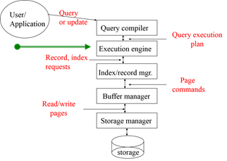
Query Execution Plans

select C.cust_name 
from Sale S, Manufacturer M, Customer C, Product P 
where M.city = 'Lima' and 
	P.prod_id = S.prod_id and 
	P.manufactr_id = M.manufactr_id and 
	S.cust_id = C.cust_id

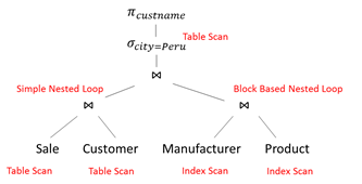
Create a Query Plan:

• logical tree
• implementation   choice at every node
• scheduling of operations.

Some operators are from relational algebra, and others (e.g., scan, group) are not.

Cost Parameters

Cost parameters 

• M = number of blocks that fit in main memory
• B(R) = number of blocks holding R
• T(R) = number of tuples in R
• V(R,a) = number of distinct values of the attribute a

Estimating the cost:

• Important in optimization (next lecture)
• Compute I/O cost only
• We compute the cost to read the tables
• We don’t compute the cost to write the result (because pipelining)

Sorting

Two pass multi-way merge sort

Step 1:

• Read M blocks at a time, sort, write
• Result: have runs of length M on disk

Step 2:

• Merge M-1 at a time, write to disk
• Result: have runs of length M(M-1)»M²

Cost: 3B(R),  Assumption: B(R) < M²

Scanning Tables

The table is clustered (I.e. blocks consists only of records from this table):

• Table-scan: if we know where the blocks are
• Index scan: if we have index to find the blocks

The table is unclustered (e.g. its records are placed on blocks with other tables)

• May need one read for each record

Clustered relation:

• Table scan:  B(R); to sort: 3B(R)
• Index scan:  B(R); to sort: B(R) or 3B(R)

Unclustered relation

• T(R); to sort: T(R) + 2B(R)

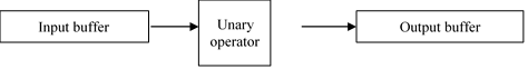
One Pass Algorithms

Selection $\sigma$(R), projection $\pi$(R)

• Both are tuple-at-a-Time algorithms
• Cost B(R)

Duplicate elimination $\delta$(R)

Need to keep a dictionary in memory:

• balanced search tree
• hash table
• etc

Cost: B(R)

Assumption: B(d(R)) <= M

Grouping: $\gamma$_{city, sum(price)} (R)

• Need to keep a dictionary in memory
• Also store the sum(price) for each city
• Cost: B(R)
• Assumption: number of cities fits in memory

Binary operations: R $\cap$ S, R $\cup$ S, R – S

• Assumption: min(B(R), B(S)) <= M
• Scan one table first, then the next, eliminate duplicates
• Cost: B(R)+B(S)

Nested Loop Joins

Tuple-based nested loop R $\bowtie$ S

R=outer relation, S=inner relation

for each tuple r in R do
   for each tuple s in S do
      if r and s join then output (r,s)

Cost: T(R) T(S),  sometimes T(R) B(S)

Block-based Nested Loop Join

for each (M-1) blocks bs of S do
   for each block br of R do
      for each tuple s in bs do
         for each tuple r in br do
            if r and s join then output(r,s)

Cost:
• Read S once: cost B(S)
• Outer loop runs B(S)/(M-1) times, and each time need to read R: costs B(S)B(R)/(M-1)
• Total cost: B(S) + B(S)B(R)/(M-1)
Notice: it is better to iterate over the smaller relation first– i.e., S smaller

Two Pass algorithms (based on sorting)

Duplicate elimination $delta$(R)

Simple idea: like sorting, but include no duplicates

Step 1: sort runs of size M, write

• Cost: 2B(R)

Step 2: merge M-1 runs, but include each tuple only once

• Cost: B(R)
• Total cost: 3B(R), Assumption: B(R)<= M²

Index-based algorithms (zero pass)

In a clustered index all tuples with the same value of the key are clustered on as few blocks as possible:

Index based selection

Selection on equality: $\sigma_{a=v}$(R)

Clustered index on a:  cost B(R)/V(R,a)

Unclustered index on a: cost T(R)/V(R,a)

Example: B(R) = 2000,  T(R) = 100,000, V(R, a) = 20, compute the cost of $\sigma_{a=v}$(R)

Cost of table scan:

• If R is clustered: B(R) = 2000 I/Os
• If R is unclustered: T(R) = 100,000 I/Os

Cost of index based selection:

• If index is clustered: B(R)/V(R,a) = 100
• If index is unclustered: T(R)/V(R,a) = 5000

Notice: when V(R,a) is small, then unclustered index is useless

Index based join

R $\bowtie$ S

Assume S has an index on the join attribute

Iterate over R, for each tuple fetch corresponding tuple(s) from S

Assume R is clustered. Cost:

• If index is clustered:  B(R) + T(R)B(S)/V(S,a)
• If index is unclustered: B(R) + T(R)T(S)/V(S,a)

Assume both R and S have a sorted index (B+ tree) on the join attribute

• Then perform a merge join (called zig-zag join)

Cost: B(R) + B(S)

Estimating Sizes

S = $\sigma_{a=c}(R)$

• T(S) can be anything from 0 to T(R) – V(R,A) + 1
• Mean value: T(S) = T(R)/V(R,A)

S = $\sigma_{a<c}(R)$

• T(S) can be anything from 0 to T(R)
• Heuristics: T(S) = T(R)/3

Estimating the size of a natural join, R join S

• When the set of A values are disjoint, then T(R join S) = 0
• When A is a key in S and a foreign key in R, then T(R join S) = T(R)
• When A has a unique value, the same in R and S, then T(R join S) = min(T(R), T(S))

In general: T(R join S) = T(R) T(S) / max(V(R,A),V(S,A))

• T(R) = 10000,  T(S) = 20000
• V(R,A) = 100,  V(S,A) = 200
• How large is R$\bowtie$S ?  = 10000*20000/200 = 1000000

Query Optimization

At the heart of the database engine

• Step 1: convert the SQL query to some logical plan
• Step 2: find a better logical plan, find an associated physical plan

SQL –> Logical Query Plans:

select a1, …, an from R1, …, Rk Where C $\rightarrow$ $\pi$a1,…,an($\sigma$C(R1 x R2 x … x Rk))

Now we have one logical plan

Algebraic laws:
                foundation for every optimization

Two approaches to optimizations:

• Rule-based (heuristics): apply laws that seem to result in cheaper plans
• Cost-based: estimate size and cost of intermediate results, search systematically for best plan

Optimizer has three things:

• Algebraic laws
• An optimization algorithm
• A cost estimator

Algebraic Laws

Commutative and Associative Laws

• R $\cup$ S = S $\cup$ R,  R $\cup$ (S $\cup$ T) = (R $\cup$ S) $\cup$ T
• R ∩ S = S ∩ R,  R ∩ (S ∩ T) = (R ∩ S) ∩ T
• R ⋈ S = S ⋈ R,  R ⋈ (S ⋈ T) = (R ⋈ S) ⋈ T

Distributive Laws

• R ⋈ (S $\cup$ T)  =  (R ⋈ S) $\cup$ (R ⋈ T)

Laws involving selection:

• s _{C AND C’}(R) = s _C(s _C’(R)) = s _C(R) ∩ s _C’(R)
• s _{C OR C’}(R) = s _C(R) $\cup$ s _C’(R)
• s _C (R ⋈ S) = s _C (R) ⋈ S

When C involves only attributes of R

• s _C (R – S) = s _C (R) – S
• s _C (R $\cup$ S) = s _C (R) $\cup$ s _C (S)
• s _C (R ∩ S)  = s _C (R) ∩ S

Rule Based Optimization

Query rewriting based on algebraic laws

Result in better queries most of the time

Heuristic number 1: Push selections down

Example:

select C.cust_name 
from Sale S, Manufacturer M, Customer C, Product P 
where M.city = 'Lima' and 
	P.prod_id = S.prod_id and 
	P.manufactr_id = M.manufactr_id and 
	S.cust_id = C.cust_id

Heuristics number 2: Sometimes push selections up, then down

When would this be helpful? Come up with an example, when pushing selections up and then back down would be helpful.